E資格向けの自習アウトプット
自分用メモ
誤差逆伝播までの流れを一旦 python実装 してみる
1.データ定義
2.順伝播(アフィン変換、ReLU)
3.コスト関数(誤差の計算)
4.誤差逆伝播
とりあえず絵にしてみる

求めたいのはパラメータの勾配
入力データの定義
実際には、入力データと正解ラベルが対になっているが、とりあえず適当に数値を用意
(例:「車の画像」と「車」というラベル)
重みとバイアスもランダムな値で
import numpy as np
x1 = np.random.rand(1,3)
t = np.array((1,0,0))
w1 = np.random.randn(3,4)
b1 = np.random.randn(4)
w2 = np.random.randn(4,3)
b2 = np.random.randn(3)
順伝播
入力データを「アフィン変換、ReLU関数」で中間層へ
ソフトマックスとで最後の
import numpy as np
def forward(x, w, b):
y = np.dot(x, w) + b
return y
def relu(x):
mask = (x <= 0)
return np.maximum(0, x), mask
def softmax(x):
x = x.T
_x = x - np.max(x)
_x = np.exp(x) / np.sum(np.exp(x), axis=0)
return _x.T
def cross_entropy_error(t, y):
delta = 1e-8
loss = -np.mean(t * np.log(y + delta))
return loss
x1 = np.random.rand(1,3)
t = np.array((1,0,0))
w1 = np.random.randn(3,4)
b1 = np.random.randn(4)
w2 = np.random.randn(4,3)
b2 = np.random.randn(3)
順伝播で出力された「誤差」を持って、勾配を逆伝播していく
順伝播の中間層で一度算出された値の再利用を一度変数に収めているが、Python の Class を使えばもっとシンプルに書くことができる
今回は敢えて各層の計算で何が必要なのかを見やすくするために、関数のみで下記揃える
def drelu(dout, mask):
dout[mask] = 0
return dout
def backward(dout, x, w):
dx = np.dot(dout, w.T)
dw = np.dot(x.T, dout)
db = np.sum(dout, axis=0)
return dx, dw, db
dout2 = y - t
dx2, dw2, db2 = backward(dout2, x2, w2)
dout1 = drelu(dx2, wmask1)
dx1, dw1, db1 = backward(dout1, x1, w1)
print('Loss: ', loss)
print('')
print('第1層の勾配')
print('w1:\n', w1)
print('b1:\n', b1)
print('')
print('第2層の勾配')
print('w2:\n', w2)
print('b2:\n', b2)
アウトプット
Loss:  0.4813766638499986

第1層の勾配
w1:
 [[-0.81608621  0.78189308 -1.98234178  0.52644459]
 [ 0.21205568  0.86098345  0.1558696  -0.62931689]
 [ 1.21615824 -0.51937533  0.33134833 -0.43714047]]
b1:
 [-0.58540344 -0.44224125  0.46466139 -0.06018246]

第2層の勾配
w2:
 [[ 0.01044176 -0.0790746  -0.70335393]
 [-0.65571456 -0.10833987  0.32557463]
 [-0.52371017  0.08358353 -0.26835567]
 [-0.77081821  0.52365595 -0.10367158]]
b2:
 [ 0.7871995   1.71908927 -1.39842447]
まとめ
誤差逆伝播を使って、パラメータの勾配を計算するところまではこんな感じ
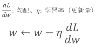
学習モデルのステップとしては、パラメータをどう更新していくかを考えていく